Spectral Binning

TauREx forward models produce spectra on a very fine native wavenumber grid — typically tens of thousands of points. Observed spectra, by contrast, rarely have more than a few hundred bins. Before comparing model to data (or just for clearer plots), the model spectrum needs to be resampled down to a coarser grid. That is the focus of this notebook, and the same technique appears directly in Fitting parameters and retrievals.

Three binners are available:

• ``SimpleBinner`` — fast nearest-neighbour binning onto any wavenumber array.

• ``FluxBinner`` — flux-conserving binning, automatically selected when binning to an observed spectrum.

• ``NativeBinner`` — a pass-through that preserves the native resolution.

More information about binning options is here, observed spectra are here, and instrument models are here.

Data Note

This notebook uses the opacity and CIA files set up in Setup and opacity data. TauREx provides the software to work with these datasets; the files themselves are third-party products from ExoMol and HITRAN.

import numpy as np
import matplotlib.pyplot as plt
from pathlib import Path
from _shared import build_transmission_model
from taurex.cia.hitrancia import EndOfHitranCIAError, HitranCIA

if not getattr(HitranCIA, "_notebook_header_patch", False):
    _original_init = HitranCIA.__init__

    def _patched_init(self, filename):
        _original_init(self, filename)
        self._pair_name = Path(filename).stem.split("_")[0]

    def _patched_read_header(self, f):
        line = f.readline()
        if line is None or line == "":
            raise EndOfHitranCIAError

        split = line.split()
        for index in range(len(split) - 4):
            try:
                start_wn = float(split[index])
                end_wn = float(split[index + 1])
                total_points_float = float(split[index + 2])
                temperature = float(split[index + 3])
                max_cia = float(split[index + 4])
            except ValueError:
                continue

            if total_points_float.is_integer():
                return start_wn, end_wn, int(total_points_float), temperature, max_cia

        raise ValueError(f"Could not parse HITRAN CIA header: {line.strip()}")

    HitranCIA.__init__ = _patched_init
    HitranCIA.read_header = _patched_read_header
    HitranCIA._notebook_header_patch = True

context = build_transmission_model(include_cia=True, include_rayleigh=True, download=False)
tm = context['tm']

print('Model ready with contributions:', [c.name for c in tm.contribution_list])

Model ready with contributions: ['Absorption', 'CIA', 'Rayleigh']

The Native Grid

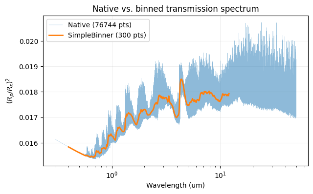
The raw output of model() is on TauREx’s internal wavenumber grid — fine enough to resolve narrow molecular lines but impractical to plot directly or compare to an observation. The cells below resample it to more manageable resolutions.

native_wn, native_rprs, _, _ = tm.model()
native_wl = 10000 / native_wn[::-1]
native_rprs = native_rprs[::-1]

print(f'Native grid: {len(native_wn)} points')
print(f'Wavelength range: {native_wl.min():.3f} to {native_wl.max():.3f} um')

Native grid: 76744 points
Wavelength range: 0.300 to 50.002 um

SimpleBinner

SimpleBinner takes any user-supplied wavenumber array and maps the native spectrum onto it using nearest-neighbour assignment. It is the fastest option and works well when bin widths are small relative to the spectral features.

The bin_model call accepts the raw tuple returned by model(), so no unpacking is needed beforehand. Equivalent parameter-file options are documented here.

from taurex.binning import SimpleBinner

# Create a logarithmic wavelength grid (0.4 - 12 um), convert to wavenumber
bin_wl = np.logspace(np.log10(0.4), np.log10(12.0), 300)
bin_wn = np.sort(10000 / bin_wl)

binner = SimpleBinner(wngrid=bin_wn)
binned_wn, binned_rprs, _, _ = binner.bin_model(tm.model(wngrid=bin_wn))
binned_wl = 10000 / binned_wn[::-1]
binned_rprs = binned_rprs[::-1]

print(f'Binned grid: {len(binned_wn)} points')

Binned grid: 300 points

plt.figure(figsize=(7, 4))
plt.plot(native_wl, native_rprs, lw=0.3, alpha=0.5, label=f'Native ({len(native_wl)} pts)')
plt.plot(binned_wl, binned_rprs, lw=2, label=f'SimpleBinner ({len(binned_wl)} pts)')
plt.xscale('log')
plt.xlabel('Wavelength (um)')
plt.ylabel('$(R_p/R_s)^2$')
plt.title('Native vs. binned transmission spectrum')
plt.legend()
plt.grid(alpha=0.2)

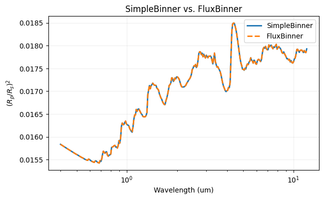
FluxBinner

FluxBinner integrates the spectrum over each output bin rather than sampling the nearest point. The result is more accurate than SimpleBinner when bin widths are comparable to or larger than the spectral features — which is typical for medium- and low-resolution instruments.

from taurex.binning import FluxBinner

flux_binner = FluxBinner(wngrid=bin_wn)
fb_wn, fb_rprs, _, _ = flux_binner.bin_model(tm.model(wngrid=bin_wn))
fb_wl = 10000 / fb_wn[::-1]
fb_rprs = fb_rprs[::-1]

plt.figure(figsize=(7, 4))
plt.plot(binned_wl, binned_rprs, lw=2, label='SimpleBinner')
plt.plot(fb_wl, fb_rprs, lw=2, ls='--', label='FluxBinner')
plt.xscale('log')
plt.xlabel('Wavelength (um)')
plt.ylabel('$(R_p/R_s)^2$')
plt.title('SimpleBinner vs. FluxBinner')
plt.legend()
plt.grid(alpha=0.2)

Binning to Real Data

When the model must be compared to an actual observation, ObservedSpectrum.create_binner() returns a FluxBinner pre-aligned to the observation’s wavelength grid. This guarantees the model and data are evaluated at exactly the same bin centres — no manual grid matching needed.

More information about observations is here, binning options are here, and instrument models are here. Fitting parameters and retrievals uses this pattern in a full retrieval.

from taurex.data.spectrum.observed import ObservedSpectrum

obs = ObservedSpectrum('observation.dat')
obs_binner = obs.create_binner()
binned_wn, binned_rprs, _, _ = obs_binner.bin_model(tm.model(obs.wavenumberGrid))

The observation file is plain text with 3–4 columns: wavelength (μm), spectral data, uncertainty, and optionally bin width.